ANOVA is not just multiple t-tests (and here's why)

The underlying idea

You’ve built three versions of a checkout page and want to know which one converts best. Version A, Version B, Version C. A natural instinct: run a t-test between A and B, then A and C, then B and C. Three tests, three p-values, done.

This approach is wrong, and the error compounds with every additional group you add.

Each t-test carries a 5% chance of a false positive at α = 0.05. When you run three tests, those error chances accumulate. The probability of at least one false positive across the three tests is approximately 14%, not 5%. Add a fourth group and you’re running six pairwise tests with a cumulative false positive rate of 26%. The more groups you test, the more likely you are to declare a difference that doesn’t exist.

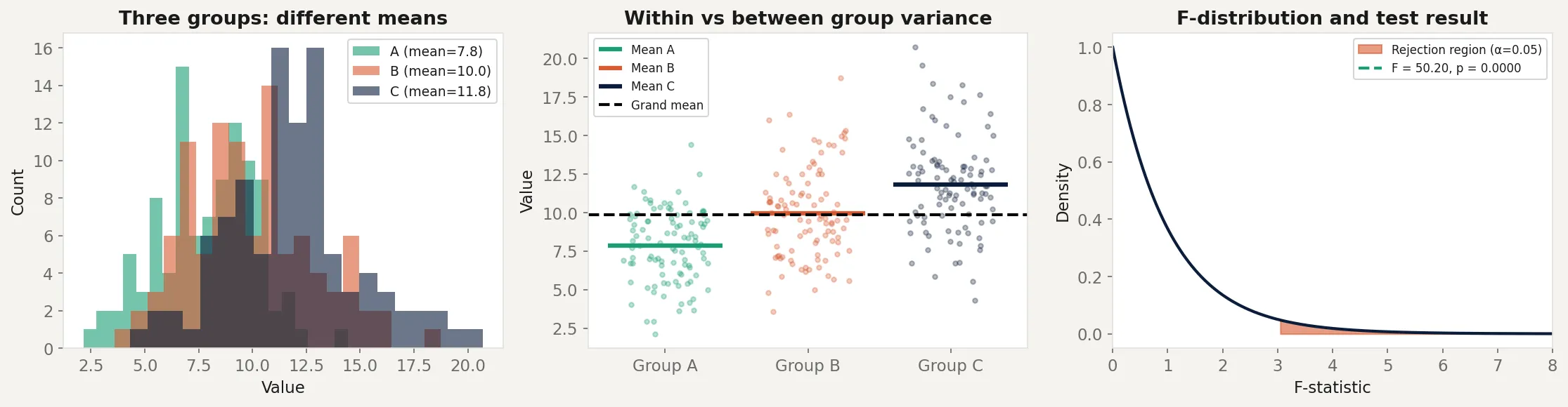
Analysis of Variance (ANOVA) solves this by testing all groups simultaneously with a single test. Instead of asking “is A different from B?” three separate times, it asks one question: “is there more variation between the groups than we’d expect from random chance?” One test, one p-value, one false positive rate controlled at α.

The counterintuitive part is in the name. ANOVA doesn’t compare means directly. It compares variances. It partitions the total variability in the data into the part explained by group membership and the part that’s just noise. When the explained part is large relative to the noise, something real is happening.

Historical root

Ronald Fisher developed ANOVA in the 1920s while working at the Rothamsted Experimental Station in England, an agricultural research institute. He was analyzing crop yield experiments where plots of land received different fertilizer treatments. The question was whether the fertilizers produced different yields, but the data was messy: soil quality varied, weather varied, and measurement error was present.

Fisher’s insight was to think about variance decomposition. The total variance in crop yields could be split into variance due to the treatment (the fertilizer) and variance due to everything else (the noise). If the treatment variance was large relative to the noise, the fertilizer was working. This ratio became the F-statistic, named after Fisher himself.

Fisher formalized ANOVA in his 1925 book Statistical Methods for Research Workers and the 1935 book The Design of Experiments. The second book introduced the concept of experimental design: randomization, blocking, and factorial designs. ANOVA and experimental design were developed together because one requires the other. A poorly designed experiment produces data that ANOVA cannot rescue.

Key assumptions

Independence of observations. Each observation must be independent of every other. If the same person appears in multiple groups (repeated measures), standard ANOVA is invalid. Repeated measures ANOVA handles this case.

Normality within groups. The observations within each group should be approximately normally distributed. ANOVA is robust to mild violations of this, especially with large sample sizes. With heavily skewed data or small samples, consider the non-parametric Kruskal-Wallis test.

Homogeneity of variance (homoscedasticity). All groups should have similar variances. ANOVA is sensitive to large differences in variance between groups. Levene’s test checks this assumption. Welch’s ANOVA relaxes it.

No interaction effects in one-way ANOVA. One-way ANOVA tests the effect of a single factor. If you have two factors (say, fertilizer type and irrigation method), their interaction can confound the results. Two-way ANOVA handles this by explicitly modeling both factors and their interaction.

The math

ANOVA decomposes the total variability in the data into two components.

Let $y_{ij}$ be the $j$-th observation in group $i$, $\bar{y}_i$ be the mean of group $i$, and $\bar{y}$ be the grand mean across all observations.

Total Sum of Squares measures overall variability:

$SS_T = \sum_{i=1}^{k} \sum_{j=1}^{n_i} (y_{ij} - \bar{y})^2$

Between-groups Sum of Squares measures variability due to group differences:

$SS_B = \sum_{i=1}^{k} n_i (\bar{y}_i - \bar{y})^2$

Within-groups Sum of Squares measures variability within each group (noise):

$SS_W = \sum_{i=1}^{k} \sum_{j=1}^{n_i} (y_{ij} - \bar{y}_i)^2$

These three quantities satisfy the decomposition:

$SS_T = SS_B + SS_W$

The F-statistic is the ratio of the between-groups variance to the within-groups variance:

$F = \frac{SS_B / (k-1)}{SS_W / (N-k)} = \frac{MS_B}{MS_W}$

where $k$ is the number of groups, $N$ is the total number of observations, $MS_B$ is the mean square between groups, and $MS_W$ is the mean square within groups.

Under the null hypothesis (all group means are equal), the F-statistic follows an F-distribution with $(k-1, N-k)$ degrees of freedom. A large F-statistic means the between-group variance is large relative to the within-group variance, which is evidence against the null.

What ANOVA doesn’t tell you: A significant F-test only tells you that at least one group mean differs from the others. It doesn’t tell you which groups differ. Post-hoc tests (Tukey’s HSD, Bonferroni, Scheffé) handle pairwise comparisons after a significant ANOVA, with corrections for multiple testing.

The code

import numpy as np
import matplotlib.pyplot as plt
from scipy import stats

rng = np.random.default_rng(42)

# Three checkout variants with different conversion rates
n_per_group = 100
group_a = rng.normal(loc=8.0, scale=3.0, size=n_per_group)
group_b = rng.normal(loc=10.0, scale=3.0, size=n_per_group)
group_c = rng.normal(loc=12.0, scale=3.0, size=n_per_group)

# One-way ANOVA
f_stat, p_value = stats.f_oneway(group_a, group_b, group_c)
print(f"F-statistic: {f_stat:.3f}")
print(f"p-value:     {p_value:.6f}")

# Manual decomposition to show the math
all_data = np.concatenate([group_a, group_b, group_c])
grand_mean = all_data.mean()
groups = [group_a, group_b, group_c]
k = len(groups)
N = len(all_data)

ss_between = sum(len(g) * (g.mean() - grand_mean)**2 for g in groups)
ss_within = sum(((g - g.mean())**2).sum() for g in groups)
ss_total = ((all_data - grand_mean)**2).sum()

ms_between = ss_between / (k - 1)
ms_within = ss_within / (N - k)
f_manual = ms_between / ms_within

print(f"\nManual decomposition:")
print(f"SS_between: {ss_between:.2f}  (df={k-1})")
print(f"SS_within:  {ss_within:.2f}  (df={N-k})")
print(f"SS_total:   {ss_total:.2f}  (df={N-1})")
print(f"F = {ms_between:.2f} / {ms_within:.2f} = {f_manual:.3f}")

# Post-hoc pairwise comparisons
from itertools import combinations
pairs = list(combinations(['A', 'B', 'C'], 2))
group_dict = {'A': group_a, 'B': group_b, 'C': group_c}

print(f"\nPairwise t-tests (no correction):")
for g1, g2 in pairs:
    t, p = stats.ttest_ind(group_dict[g1], group_dict[g2])
    sig = "significant" if p < 0.05 else "not significant"
    print(f"  {g1} vs {g2}: p={p:.4f} ({sig})")

# Show the multiple comparison problem
n_tests = 3
alpha = 0.05
family_wise = 1 - (1 - alpha) ** n_tests
print(f"\nWith {n_tests} tests at alpha={alpha}:")
print(f"Family-wise error rate: {family_wise:.3f} (not {alpha})")
print(f"Bonferroni correction:  alpha per test = {alpha/n_tests:.4f}")

The F-test gives a single p-value for the comparison of all three groups. The manual decomposition verifies the math: SS_between + SS_within = SS_total. The pairwise section shows all three pairs are individually significant, but the family-wise error rate is 14%, not 5%. The Bonferroni correction shows the adjusted threshold needed to maintain the correct family-wise rate.

Business application

Multivariate testing (A/B/C/n tests). When you have more than two variants, ANOVA is the right first test. It tells you whether any variant produces a different result before you start comparing specific pairs. If the ANOVA F-test is not significant, you stop. No post-hoc comparisons needed. If it is significant, run post-hoc tests with appropriate corrections.

Clinical trials with multiple treatment arms. Drug trials often compare a new drug against a placebo and against an existing standard of care. Three groups means ANOVA first, then pairwise comparisons. Running three t-tests instead inflates the false positive rate and doesn’t respect the family-wise error structure.

Manufacturing quality control. If parts come off three different production lines and you want to know whether the lines produce parts of the same quality, ANOVA tests whether the variation between lines exceeds the variation within lines. A significant result prompts investigation of which line is the outlier.

When to use ANOVA versus alternatives. Use one-way ANOVA when you have one categorical factor and a continuous outcome with three or more groups. Use two-way ANOVA when you have two categorical factors. Use repeated measures ANOVA when the same subjects appear in multiple groups (before/after designs, time series with the same participants). Use Kruskal-Wallis when the normality assumption fails badly. Use Welch’s ANOVA when group variances are very different. Use regression when your factor is continuous rather than categorical. ANOVA and regression are mathematically equivalent for categorical predictors, but regression generalizes further.