The bias-variance tradeoff controls every model you'll ever build

The underlying idea

You’re building a model to predict house prices. You could fit a straight line through the data. It’ll miss a lot of detail, but it’ll be stable: give it new data and the predictions won’t change much. Or you could fit a curve that passes through every single data point. It captures every detail perfectly, but it’s fragile: give it new data and the predictions will be wildly different.

The straight line has high bias (it systematically gets the answer wrong because it’s too simple) and low variance (it gives consistent answers across different datasets). The wiggly curve has low bias (it can fit any pattern) and high variance (it’s fitting noise, not signal, so it changes dramatically with new data).

This is the bias-variance tradeoff. Every predictive model lives on a spectrum between these two extremes. Too simple and it misses real patterns. Too complex and it memorizes noise. The goal isn’t to eliminate both. You can’t. The goal is to find the point where their combined effect on prediction error is smallest.

This tradeoff is the reason regularization exists. It’s the reason we use cross-validation. It’s the reason a random forest (many simple trees) often beats a single deep tree. Every technique in machine learning is, at some level, a strategy for managing this tradeoff.

Historical root

The bias-variance decomposition was formalized by Stuart Geman and Donald Geman in 1992, though the underlying ideas are much older. The tension between model simplicity and model complexity has been a central problem in statistics since at least the early 20th century.

Ronald Fisher’s work on maximum likelihood estimation in the 1920s implicitly dealt with bias. Fisher showed that some estimators are biased (they systematically miss the true value) but can still be useful if their variance is low enough. The concept of mean squared error (MSE = bias squared + variance) gives this tradeoff a single number to optimize.

The machine learning community made the tradeoff famous in the 1990s and 2000s as overfitting became the dominant practical problem. Vapnik’s structural risk minimization (the theory behind SVMs) and Breiman’s work on bagging and random forests were both direct responses to the variance problem. The entire regularization literature (ridge regression, lasso, dropout in neural networks) is a toolkit for trading increased bias for decreased variance.

More recently, the “double descent” phenomenon has complicated the picture. Very large neural networks can sometimes decrease both bias and variance simultaneously by being so overparameterized that they find smooth interpolations of the training data. This doesn’t invalidate the tradeoff. It means the tradeoff operates differently in very high-dimensional spaces than classical theory predicted.

Key assumptions

The decomposition applies to squared error loss. The clean “MSE = bias squared + variance” formula holds for squared error. With other loss functions (absolute error, log loss), the decomposition exists but takes different forms and the tradeoff isn’t as clean.

The true function exists and is fixed. The decomposition assumes there’s a true underlying relationship between inputs and outputs, and that your model is trying to approximate it. If the relationship is changing over time (concept drift), both bias and variance become moving targets.

Noise is irreducible. The decomposition includes a third term: irreducible error (noise). This is the randomness inherent in the data that no model can capture. If measurement error is large or the outcome is genuinely unpredictable given the inputs, no amount of model tuning will get past this floor.

Variance is measured across datasets. Variance in this context doesn’t mean the variance of the data (that’s A4). It means the variance of the model’s predictions across different training sets drawn from the same population. A high-variance model gives very different predictions depending on which training data it happened to see.

The math

The mean squared error of a model’s prediction $\hat{f}(x)$ at a point $x$ can be decomposed into three terms:

$\text{MSE}(x) = \text{Bias}^2(x) + \text{Var}(x) + \sigma^2$

where:

Bias measures the systematic error. It’s the difference between the expected prediction (averaged over all possible training sets) and the true value:

$\text{Bias}(x) = E[\hat{f}(x)] - f(x)$

A model with high bias consistently predicts values that are too high or too low, regardless of the training data. Linear regression on a nonlinear problem has high bias.

Variance measures the sensitivity to the training data. It’s how much the prediction at $x$ changes across different training sets:

$\text{Var}(x) = E\left[(\hat{f}(x) - E[\hat{f}(x)])^2\right]$

A model with high variance gives different predictions depending on which training set it saw. A deep decision tree has high variance because small changes in the training data produce completely different tree structures.

Irreducible error $\sigma^2$ is the noise in the data. It’s the variance of the true outcome around the true function. No model can reduce this. If $\sigma^2$ is large, your model’s MSE will be high even if bias and variance are both zero.

The tradeoff works like this: as you increase model complexity, bias typically decreases (the model can represent more patterns) and variance typically increases (the model becomes more sensitive to the specific training data). The total error follows a U-shaped curve, and the minimum of that curve is the sweet spot.

The code

This script demonstrates the bias-variance tradeoff using polynomial regression at different complexities.

import numpy as np
import matplotlib.pyplot as plt
from sklearn.preprocessing import PolynomialFeatures
from sklearn.linear_model import LinearRegression
from sklearn.pipeline import make_pipeline

rng = np.random.default_rng(42)

# True function: a gentle curve
def true_function(x):
    return np.sin(2 * x) + 0.5 * x

# Generate multiple training sets to measure bias and variance
n_datasets = 200
n_train = 30
n_test = 100
x_test = np.linspace(0, 5, n_test).reshape(-1, 1)
y_true = true_function(x_test.ravel())

degrees = [1, 3, 5, 10, 15]
fig, axes = plt.subplots(2, 3, figsize=(15, 9))

# Top row: show fits for three complexity levels
for idx, degree in enumerate([1, 5, 15]):
    ax = axes[0, idx]
    ax.plot(x_test, y_true, 'k-', linewidth=2, label="True function")

    for i in range(20):  # show 20 fits
        x_train = rng.uniform(0, 5, n_train).reshape(-1, 1)
        y_train = true_function(x_train.ravel()) + rng.normal(0, 0.5, n_train)
        model = make_pipeline(PolynomialFeatures(degree), LinearRegression())
        model.fit(x_train, y_train)
        y_pred = model.predict(x_test)
        ax.plot(x_test, y_pred, alpha=0.15, color="steelblue")

    ax.set_title(f"Degree {degree}")
    ax.set_ylim(-3, 6)
    if idx == 0:
        ax.set_ylabel("y")

# Bottom row: compute bias^2, variance, and MSE across degrees
all_degrees = range(1, 16)
bias_sq_list = []
var_list = []
mse_list = []

for degree in all_degrees:
    predictions = np.zeros((n_datasets, n_test))

    for i in range(n_datasets):
        x_train = rng.uniform(0, 5, n_train).reshape(-1, 1)
        y_train = true_function(x_train.ravel()) + rng.normal(0, 0.5, n_train)
        model = make_pipeline(PolynomialFeatures(degree), LinearRegression())
        model.fit(x_train, y_train)
        predictions[i] = model.predict(x_test).ravel()

    mean_pred = predictions.mean(axis=0)
    bias_sq = np.mean((mean_pred - y_true) ** 2)
    variance = np.mean(predictions.var(axis=0))
    mse = np.mean((predictions - y_true) ** 2)

    bias_sq_list.append(bias_sq)
    var_list.append(variance)
    mse_list.append(mse)

# Plot decomposition
ax = axes[1, 0]
ax.plot(list(all_degrees), bias_sq_list, 'o-', label="Bias²", color="coral")
ax.plot(list(all_degrees), var_list, 's-', label="Variance", color="steelblue")
ax.plot(list(all_degrees), mse_list, '^-', label="MSE (total)", color="black")
ax.axhline(y=0.25, color="gray", linestyle=":", label="Noise (σ²=0.25)")
ax.set_xlabel("Polynomial degree")
ax.set_ylabel("Error")
ax.set_title("Bias-variance decomposition")
ax.legend(fontsize=8)

# Hide unused subplots
axes[1, 1].axis("off")
axes[1, 2].axis("off")

plt.tight_layout()
plt.savefig("bias_variance.png", dpi=150)
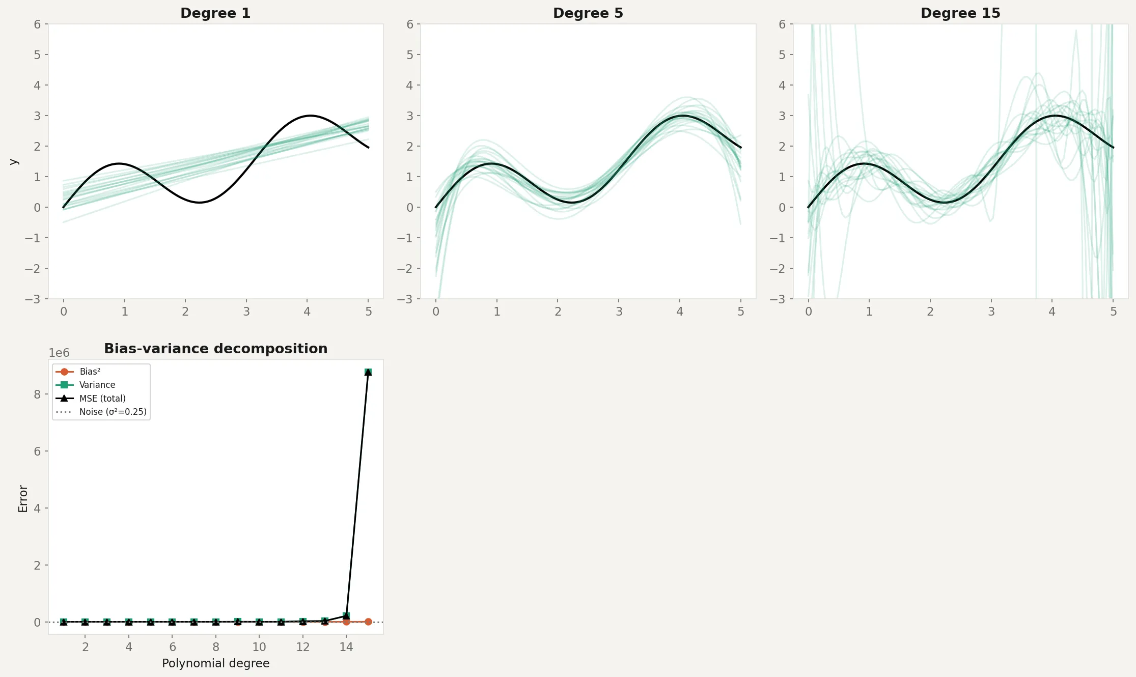
plt.show()

The top row shows 20 model fits on different training sets at three complexity levels. Degree 1 (linear) produces consistent but wrong predictions: high bias, low variance. Degree 5 produces predictions that track the true function reasonably well: the sweet spot. Degree 15 produces predictions that swing wildly between datasets: low bias on average, but enormous variance.

The bottom-left panel shows the decomposition. As polynomial degree increases, bias drops (the model can represent the true curve) but variance rises (the model starts fitting noise). Total MSE follows a U-shape. The minimum is around degree 4-5, which matches the visual impression from the top row. The gray dotted line shows the noise floor ($\sigma^2 = 0.25$), which no model can beat.

Business application

Model selection. The bias-variance tradeoff is the reason you don’t always pick the most complex model. A gradient boosted model with 1,000 trees might have lower training error than one with 100 trees, but higher test error because it’s fitting noise. Cross-validation exists specifically to estimate where on the U-curve your model sits.

Regularization. Ridge regression, lasso, and elastic net all add a penalty for model complexity. This deliberately increases bias in exchange for decreased variance. The regularization parameter controls the tradeoff. Too much regularization: underfitting (high bias). Too little: overfitting (high variance). The optimal value is found through cross-validation.

Ensemble methods. Random forests reduce variance by averaging many high-variance trees. Each individual tree overfits, but their average doesn’t. Bagging works because the variance of an average is lower than the variance of individual predictions (this connects directly to the standard error formula from A4: $s / \sqrt{n}$). Boosting takes the opposite approach: it starts with a high-bias model and sequentially reduces bias by correcting residuals.

Feature engineering. Adding more features to a model can reduce bias (more information to work with) but increase variance (more opportunities to fit noise). Removing irrelevant features reduces variance without increasing bias. This is why feature selection and dimensionality reduction (PCA) are standard preprocessing steps.

When the tradeoff doesn’t apply cleanly. Very large neural networks appear to violate the classical tradeoff. They have enough parameters to memorize the training data (zero bias) yet still generalize well. Current research suggests this happens because of implicit regularization in gradient descent and the geometry of high-dimensional loss surfaces. The tradeoff still exists in principle. The practical boundaries of where it bites have shifted with scale.