Chi-square tests: how to make decisions from categories

The underlying idea

Most statistical tests assume you’re measuring something on a continuous scale. Revenue, height, conversion rate. But a lot of the data that actually matters in business is categorical. Did the customer click yes or no? Which product category did they buy? Which region are they from? Did the treatment work or not?

When your data is counts of categories, not measurements, the t-test and ANOVA don’t apply. The chi-square test is the tool for this situation. It answers two different questions depending on how you use it.

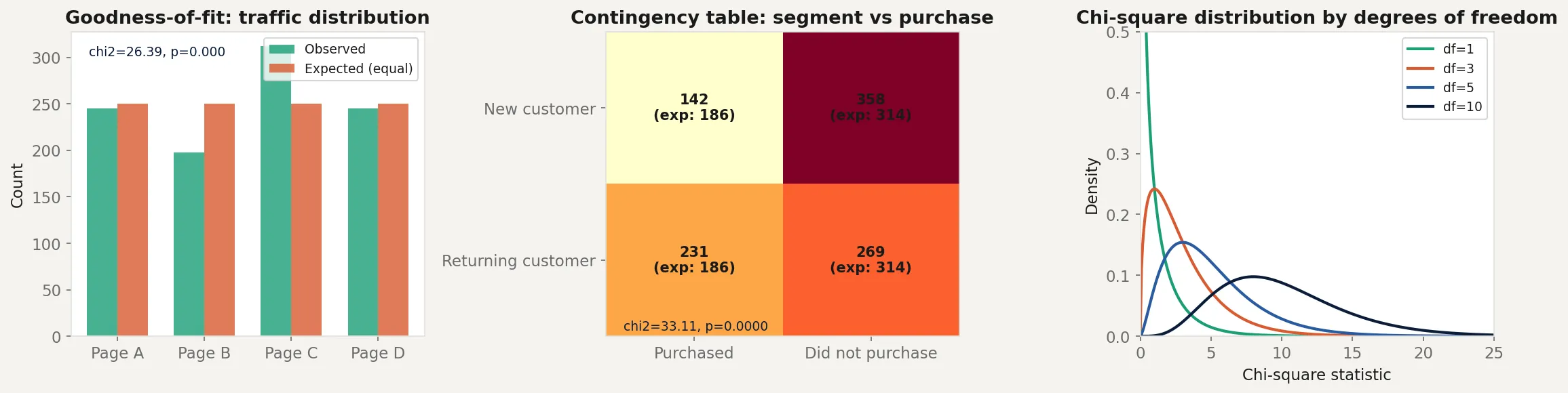
The goodness-of-fit test asks: does the distribution of a single categorical variable match an expected distribution? If you expect equal traffic across four landing pages but observe very unequal numbers, is that surprising or just random variation?

The test of independence asks: are two categorical variables related? If you cross-tabulate customer segment (new vs returning) against purchase outcome (bought vs did not buy), is segment associated with purchase behavior, or are they independent?

Both tests use the same core idea: compare what you observed with what you would expect if your null hypothesis were true. When the gap between observed and expected is large enough relative to what random variation could explain, you reject the null.

Historical root

Karl Pearson introduced the chi-square test in 1900, making it one of the oldest formal statistical tests still in widespread use. Pearson was working on problems in evolutionary biology and needed a way to test whether observed frequency distributions matched theoretical ones.

His paper introduced the chi-square statistic and its distribution. The paper was a landmark because it provided a rigorous method for comparing observed and expected counts, something that had previously been done informally.

Pearson had a complicated relationship with Ronald Fisher, who later showed that Pearson had made an error in the degrees of freedom for the test of independence. Fisher corrected it in 1922, reducing the degrees of freedom by one for contingency tables. The dispute lasted years and was never fully resolved between the two men.

The chi-square distribution itself predates Pearson’s application of it. Friedrich Helmert derived it in 1875 in the context of measurement errors, and Ernst Abbe had worked with it even earlier. Pearson’s contribution was connecting this mathematical distribution to a practical testing procedure.

Key assumptions

Independence of observations. Each observation must be independent. You cannot include the same person twice in the count. If observations are clustered (students within classrooms, patients within hospitals), standard chi-square is invalid.

Expected cell counts are large enough. The chi-square approximation works poorly when expected counts are very small. The common rule is that all expected cell counts should be at least 5. With smaller counts, Fisher’s exact test is more appropriate.

Categorical data only. The chi-square test requires counts of categories. If you have continuous data that you have binned into categories, the result depends on your choice of bins, which introduces researcher degrees of freedom. Be careful.

The categories are mutually exclusive and exhaustive. Each observation belongs to exactly one category. No overlaps, no missing categories.

Sample size is fixed. The marginal totals in a contingency table should be determined by the data collection process, not by the analysis. If you stopped data collection when you had enough to get significance, your p-value is invalid.

The math

For both tests, the chi-square statistic has the same form:

$\chi^2 = \sum_{i} \frac{(O_i - E_i)^2}{E_i}$

where $O_i$ is the observed count in category $i$ and $E_i$ is the expected count under the null hypothesis.

Goodness-of-fit test. If you have $k$ categories and expect proportions $p_1, p_2, \ldots, p_k$ under the null, the expected count for category $i$ with total $n$ observations is $E_i = n \cdot p_i$. The test statistic follows a chi-square distribution with $k - 1$ degrees of freedom.

Test of independence. For a contingency table with $r$ rows and $c$ columns, the expected count for cell $(i, j)$ under independence is:

$E_{ij} = \frac{(\text{row } i \text{ total}) \times (\text{column } j \text{ total})}{n}$

The test statistic follows a chi-square distribution with $(r-1)(c-1)$ degrees of freedom.

The degrees of freedom reflect how many free parameters you have after estimating the marginal totals from the data. More cells mean more degrees of freedom, and the same chi-square statistic is less surprising with more degrees of freedom.

The p-value is the probability of observing a chi-square statistic at least as large as yours if the null hypothesis were true. Large chi-square values mean the observed and expected counts are far apart. They live in the right tail of the chi-square distribution.

The code

import numpy as np
from scipy import stats

rng = np.random.default_rng(42)

# --- Goodness of fit: equal traffic across pages? ---
observed_traffic = np.array([245, 198, 312, 245])
n_total = observed_traffic.sum()
expected_equal = np.full(4, n_total / 4)

chi2_gof, p_gof = stats.chisquare(observed_traffic, expected_equal)
print("Goodness-of-fit test (equal traffic across 4 pages):")
print(f"  Observed: {observed_traffic}")
print(f"  Expected: {expected_equal}")
print(f"  chi2 = {chi2_gof:.3f}, p = {p_gof:.4f}")

# --- Test of independence: customer segment vs purchase ---
# Rows: New customers, Returning customers
# Columns: Purchased, Did not purchase
contingency = np.array([
    [142, 358],
    [231, 269]
])

chi2_ind, p_ind, dof, expected_ind = stats.chi2_contingency(contingency)
print(f"\nTest of independence (segment vs purchase):")
print(f"  Observed:\n{contingency}")
print(f"  Expected:\n{expected_ind.astype(int)}")
print(f"  chi2 = {chi2_ind:.3f}, p = {p_ind:.4f}, df = {dof}")

# Cramer's V: effect size for chi-square
n = contingency.sum()
cramers_v = np.sqrt(chi2_ind / (n * (min(contingency.shape) - 1)))
print(f"  Cramer's V = {cramers_v:.3f}")

# Manual verification
chi2_manual = 0
for i in range(2):
    for j in range(2):
        chi2_manual += (contingency[i,j] - expected_ind[i,j])**2 / expected_ind[i,j]
print(f"\nManual chi2 = {chi2_manual:.3f} (matches scipy: {np.isclose(chi2_manual, chi2_ind)})")

The goodness-of-fit test checks whether the four landing pages get equal traffic. Page C has noticeably more visits than the others. The chi-square statistic measures whether that imbalance is large enough to be unlikely under the null of equal distribution.

The independence test checks whether customer segment is associated with purchase behavior. The expected values under independence are computed from the row and column totals. Returning customers purchase at a higher rate than new customers in the observed data. The chi-square statistic tests whether that gap exceeds what you would expect from sampling variation alone. Cramer’s V gives the effect size on a 0 to 1 scale, making the result interpretable regardless of sample size.

Business application

Product analytics. You have four notification types and want to know if users engage equally with all of them. A goodness-of-fit test with equal expected proportions answers this in one test. If significant, look at which categories are above or below their expected counts to understand where the imbalance is.

Marketing attribution. You want to know whether the channel a customer came through (organic, paid, email, referral) is associated with whether they make a repeat purchase. A contingency table of channel by repeat purchase, tested with chi-square, answers this directly.

Fraud detection. Transaction categories that appear far more or less often than historical norms can signal unusual activity. A goodness-of-fit test against historical proportions flags anomalies without requiring continuous measurements.

A/B testing with binary outcomes. When your outcome is categorical (clicked vs did not click, bought vs did not buy), chi-square tests the association between variant assignment and outcome. For 2x2 tables, this is mathematically equivalent to a z-test for proportions, but chi-square generalizes naturally to more than two variants or more than two outcome categories.

What chi-square cannot tell you. A significant chi-square result tells you that the observed and expected distributions differ, or that two variables are associated. It doesn’t tell you the direction or magnitude of the relationship without further analysis. For 2x2 tables, look at the odds ratio. For larger tables, examine the standardized residuals for each cell to see which categories are driving the deviation. And with large enough samples, trivially small associations will appear significant. Always pair a significant result with an effect size measure like Cramer’s V.