Decision trees learn by asking the right questions

The underlying idea

Imagine you’re a doctor trying to diagnose a patient. You don’t run every possible test at once. You start with the question that splits the possibilities most effectively. Fever? That rules out half the conditions immediately. Then you ask the next most useful question given the answer to the first one. Each question narrows the field until you reach a diagnosis.

A decision tree does exactly this with data. It looks at your features and finds the single split that best separates the target variable into purer groups. Then it repeats the process on each resulting group, and again, and again, until it reaches a stopping point. The output is a tree of if-then rules that you can read top to bottom.

What makes decision trees unusual in machine learning is that the result is interpretable. You can hand a trained decision tree to a business stakeholder and they can trace any prediction back through a chain of concrete rules. Good luck extracting that from a neural network with 50 million parameters.

Historical root

The modern decision tree traces back to two independent lines of work. On the statistics side, Morgan and Sonquist introduced AID (Automatic Interaction Detection) in 1963 at the University of Michigan. They wanted to find which survey variables best explained differences in income, and they did it by recursively splitting the data.

On the machine learning side, Ross Quinlan developed ID3 in 1986, followed by C4.5 in 1993. Quinlan’s contribution was formalizing the splitting criterion using information theory. He borrowed Shannon’s concept of entropy to measure how “mixed” a group was, then chose splits that reduced that mixture the most. C4.5 became one of the most widely cited algorithms in machine learning.

Leo Breiman and colleagues took a different approach with CART (Classification and Regression Trees) in 1984. CART used the Gini impurity index instead of entropy and produced binary splits only. Breiman later built on CART to create random forests in 2001, which solved many of the single tree’s weaknesses by combining hundreds of trees trained on random subsets of the data.

Key assumptions

Decision trees have surprisingly few formal assumptions, which is part of their appeal. But they have important practical limitations that act like hidden assumptions.

No assumed relationship between features and target. Unlike linear regression, a decision tree doesn’t assume the relationship is linear, additive, or any particular shape. It can capture interactions and nonlinearities automatically.

Feature scale doesn’t matter. Trees split on thresholds (“is age > 35?”), so whether you measure income in dollars or thousands of dollars changes nothing. No normalization needed.

Greedy splitting is good enough. The algorithm picks the best split at each step without looking ahead. It never asks “would a worse split now lead to a better tree overall?” This greedy approach works well in practice but means the tree you get isn’t globally optimal. Two datasets with minor differences can produce very different trees.

Sufficient data at each leaf. If the tree grows too deep, leaf nodes end up with very few observations. Predictions based on three data points are unreliable. Pruning or setting a minimum leaf size prevents this, but you have to actually do it.

Sensitive to class imbalance. If 95% of your data belongs to one class, the tree can achieve 95% accuracy by predicting that class everywhere. The splitting criteria technically still work, but the tree will barely explore the minority class. Resampling, class weights, or adjusted splitting thresholds help.

The math

A decision tree needs a way to measure how “good” a split is. Two metrics dominate: Gini impurity and entropy. Both measure the same thing (how mixed the classes are in a node) and usually produce similar trees.

Gini impurity for a node with $K$ classes:

$$G = 1 - \sum_{k=1}^{K} p_k^2$$

where $p_k$ is the proportion of samples belonging to class $k$ in that node. If a node is perfectly pure (all one class), $G = 0$. If classes are evenly split (binary case, 50/50), $G = 0.5$.

Entropy (information-theoretic version):

$$H = -\sum_{k=1}^{K} p_k \log_2 p_k$$

A perfectly pure node has $H = 0$. A 50/50 binary split gives $H = 1$ bit.

When evaluating a potential split, the algorithm computes the information gain (or Gini reduction):

$$\text{Gain} = H(\text{parent}) - \sum_{j} \frac{n_j}{n} H(\text{child}_j)$$

where the sum runs over the child nodes created by the split, $n_j$ is the number of samples in child $j$, and $n$ is the total in the parent. The split with the highest gain wins.

The algorithm checks every feature and every possible threshold for that feature. For a continuous variable with 100 unique values, that’s 99 possible splits for that feature alone. Multiply by the number of features and you see why training is computationally straightforward but not free.

The code

Here’s a complete example: training a decision tree, inspecting what it learned, and understanding where it breaks down.

import numpy as np
from sklearn.datasets import make_classification
from sklearn.tree import DecisionTreeClassifier, export_text
from sklearn.model_selection import train_test_split

rng = np.random.default_rng(42)

# Create a dataset with 2 informative features and 1 noisy one
X, y = make_classification(
    n_samples=500,
    n_features=3,
    n_informative=2,
    n_redundant=0,
    n_clusters_per_class=1,
    random_state=42
)

X_train, X_test, y_train, y_test = train_test_split(
    X, y, test_size=0.3, random_state=42
)

# Unpruned tree (will overfit)
tree_deep = DecisionTreeClassifier(random_state=42)
tree_deep.fit(X_train, y_train)
print(f"Unpruned depth:    {tree_deep.get_depth()}")
print(f"Unpruned train acc: {tree_deep.score(X_train, y_train):.3f}")
print(f"Unpruned test acc:  {tree_deep.score(X_test, y_test):.3f}")

# Pruned tree (controlled complexity)
tree_pruned = DecisionTreeClassifier(
    max_depth=4,
    min_samples_leaf=10,
    random_state=42
)
tree_pruned.fit(X_train, y_train)
print(f"\nPruned depth:      {tree_pruned.get_depth()}")
print(f"Pruned train acc:   {tree_pruned.score(X_train, y_train):.3f}")
print(f"Pruned test acc:    {tree_pruned.score(X_test, y_test):.3f}")

# Print the pruned tree's rules
print("\nDecision rules:")
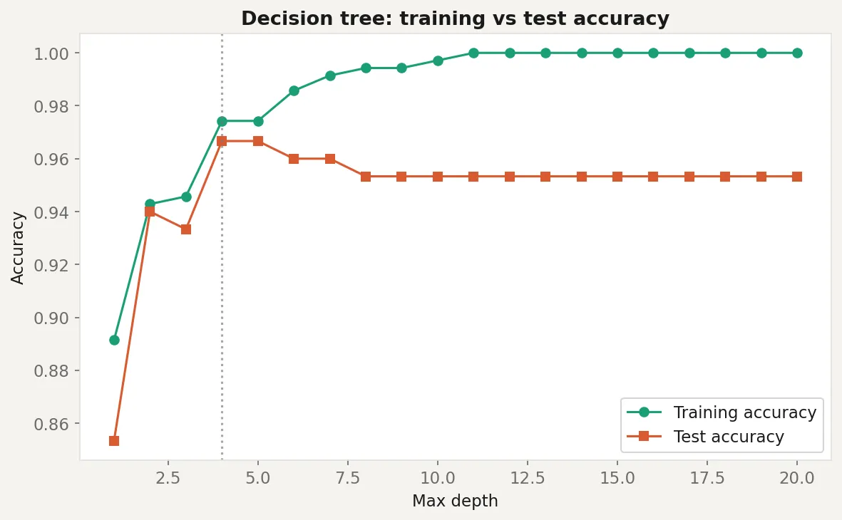
print(export_text(tree_pruned, feature_names=["feat_0", "feat_1", "noise"]))

The unpruned tree will score near-perfect on training data and noticeably worse on test data. That gap is overfitting in action. The pruned version sacrifices a few points of training accuracy to hold up better on new data. The printed rules show exactly what the tree learned, and you’ll likely notice that the noise feature barely appears. The tree figured out which features carry signal and which don’t, without you telling it.

Business application

Credit scoring and loan approval. Decision trees are common in financial services because regulators require explainability. A loan officer can point to the exact rule chain that produced a decision. “This applicant was rejected because their debt-to-income ratio exceeded 0.45 and their credit history was under 3 years.”

Customer segmentation. Trees naturally produce segments. Train a tree to predict churn, then look at the leaf nodes. Each leaf is a customer segment defined by concrete feature thresholds, ready to hand to a marketing team without any translation.

Medical diagnosis support. Trees mirror how clinicians think: sequential questions that narrow the diagnosis. They’ve been used in triage protocols and clinical decision support systems where interpretability is non-negotiable.

When NOT to use a single tree. Don’t rely on one decision tree for high-stakes predictions. Individual trees have high variance: small changes in the training data can produce completely different tree structures. This is why ensemble methods exist. Random forests (typically 100 to 500 trees, each trained on a bootstrapped sample with random feature subsets) and gradient boosting (trees trained sequentially to correct each other’s errors) consistently outperform single trees. Use a single tree when you need interpretability. Use an ensemble when you need accuracy. If you need both, look at methods like SHAP values applied on top of an ensemble.