p-values are not what you were taught

The underlying idea

You run an experiment. You compute a p-value of 0.03. You declare the result significant. Your colleague asks what that means, and you say “there’s a 3% chance the result was due to random chance.” That interpretation is wrong. It’s the most common wrong interpretation in all of applied statistics, and it leads to real decisions being made on false grounds.

A p-value is the probability of observing data at least as extreme as what you observed, assuming the null hypothesis is true. It is not the probability that your result is due to chance. It is not the probability that the null hypothesis is true. It is not the probability that your finding will replicate.

The p-value is a statement about the data given a hypothesis, not about the hypothesis given the data. That reversal is the entire source of confusion.

Knowing what a p-value isn’t is as important as knowing what it is. The threshold of 0.05 that dominates scientific publishing is arbitrary. The decision to declare something “significant” or “not significant” based on crossing that threshold is a categorical choice imposed on a continuous quantity. And the practice of testing many hypotheses while reporting only the ones that cross the threshold can make any null result look significant if you run enough tests.

Historical root

Two separate statistical traditions gave us the p-value, and the hybrid that practitioners use today is a confused merger of both.

Ronald Fisher introduced the p-value in his 1925 book Statistical Methods for Research Workers as a continuous measure of evidence against the null hypothesis. For Fisher, p = 0.03 meant “moderate evidence against H₀.” He explicitly rejected the idea of a fixed threshold. A small p-value should prompt further investigation, not a declaration of truth.

Jerzy Neyman and Egon Pearson introduced a competing framework in 1933 based on decision theory. Their approach required specifying two hypotheses (null and alternative), a significance level α chosen in advance, and a power level. The output was a binary decision: reject or do not reject. The significance level α controlled the long-run false positive rate across many experiments, not the strength of evidence in any single one.

Practitioners in the 1940s and 1950s merged these two frameworks without reconciling their philosophical differences. Fisher’s p-value became the number computed. Neyman-Pearson’s α = 0.05 became the threshold applied to it. The result is a procedure that neither Fisher nor Neyman-Pearson would fully endorse, yet it became the standard.

Fisher and Neyman-Pearson had a bitter personal feud that lasted decades. Fisher called Neyman-Pearson’s approach “infantile” and “childish.” Neyman called Fisher’s framework incoherent. Both were partly right. The confusion in practice reflects the unresolved disagreement between the founders.

Key assumptions

The null hypothesis is specified in advance. A p-value is only meaningful if the null hypothesis was chosen before seeing the data. If you look at the data and then construct a hypothesis that the data would reject, any resulting p-value is invalid. This is the core of p-hacking.

A single test is being performed. If you test 20 independent hypotheses, each at α = 0.05, you expect one false positive even if all nulls are true. The p-value from any individual test doesn’t account for the others. Multiple testing corrections (Bonferroni, Benjamini-Hochberg) are required when testing many hypotheses simultaneously.

The test statistic has the correct null distribution. The p-value is computed by comparing your observed statistic against what you’d expect under the null. If the null distribution is wrong (wrong assumptions about normality, independence, or variance), the p-value is wrong.

The test was not peeked at. Computing a p-value while data collection is ongoing and stopping when p < 0.05 is statistically invalid. Sequential testing methods exist precisely for this case.

The math

For a test statistic $T$ and observed value $t_{obs}$, the two-tailed p-value is:

$p = P(|T| \geq |t_{obs}| \mid H_0 \text{ is true})$

This is the area in the tails of the null distribution beyond your observed statistic. Nothing more.

The connection to the significance level α works like this. Before the experiment, you choose α (the maximum false positive rate you’ll tolerate). After computing the p-value, you compare:

$\text{Reject } H_0 \text{ if } p \leq \alpha$

This decision rule guarantees that across many experiments where $H_0$ is true, you’ll incorrectly reject at most a fraction α of the time.

What p-values cannot tell you:

$P(H_0 \text{ is true} \mid \text{data}) \neq p\text{-value}$

The left side is what practitioners want. It’s the probability the null is true given the data. The p-value is the reverse: the probability of the data given that the null is true. These are related through Bayes’ theorem, but the conversion requires a prior probability for $H_0$, which the frequentist framework doesn’t provide.

The multiple testing problem: if you run $m$ independent tests each at level α, the probability of at least one false positive is:

$P(\text{at least one false positive}) = 1 - (1-\alpha)^m$

At α = 0.05 and $m = 20$: $1 - (0.95)^{20} \approx 0.64$. A 64% chance of at least one false positive from testing 20 things, even if none of them are true effects.

The code

This script demonstrates three things: what a p-value actually measures, how p-hacking works, and how the multiple testing problem inflates false positives.

import numpy as np
import matplotlib.pyplot as plt
from scipy import stats

rng = np.random.default_rng(42)

fig, axes = plt.subplots(1, 3, figsize=(15, 4))

# --- Panel 1: p-value as tail area ---
x = np.linspace(-4, 4, 300)
null_dist = stats.norm.pdf(x)
observed = 2.1
p_val = 2 * (1 - stats.norm.cdf(abs(observed)))

axes[0].plot(x, null_dist, color='#0B1D3A', linewidth=2)
axes[0].fill_between(x, null_dist, where=(x >= abs(observed)),
                     color='#D85A30', alpha=0.7, label=f'p-value = {p_val:.3f}')
axes[0].fill_between(x, null_dist, where=(x <= -abs(observed)),
                     color='#D85A30', alpha=0.7)
axes[0].axvline(x=observed, color='#D85A30', linestyle='--', linewidth=1.5)
axes[0].axvline(x=-observed, color='#D85A30', linestyle='--', linewidth=1.5)
axes[0].set_title('p-value as tail probability under H₀')
axes[0].set_xlabel('Test statistic')
axes[0].set_ylabel('Density')
axes[0].legend(fontsize=9)

# --- Panel 2: p-hacking simulation ---
n_experiments = 1000
n_per_experiment = 30
p_values_null = []

for _ in range(n_experiments):
    group_a = rng.normal(0, 1, n_per_experiment)
    group_b = rng.normal(0, 1, n_per_experiment)  # same distribution
    _, p = stats.ttest_ind(group_a, group_b)
    p_values_null.append(p)

p_values_null = np.array(p_values_null)
false_positive_rate = (p_values_null < 0.05).mean()

axes[1].hist(p_values_null, bins=20, density=True, alpha=0.7, color='#1B9E77')
axes[1].axvline(x=0.05, color='#D85A30', linestyle='--', linewidth=2,
                label=f'α = 0.05 ({false_positive_rate:.1%} false positives)')
axes[1].set_title('p-values when H₀ is TRUE\n(1000 experiments)')
axes[1].set_xlabel('p-value')
axes[1].set_ylabel('Density')
axes[1].legend(fontsize=9)

# --- Panel 3: Multiple testing inflation ---
m_tests = range(1, 101)
fpr = [1 - (0.95 ** m) for m in m_tests]

axes[2].plot(list(m_tests), fpr, color='#0B1D3A', linewidth=2)
axes[2].axhline(y=0.05, color='#D85A30', linestyle='--', linewidth=1.5,
                label='5% target rate')
axes[2].axhline(y=0.64, color='#2A5BA0', linestyle=':', linewidth=1.5,
                label='64% at m=20 tests')
axes[2].axvline(x=20, color='#2A5BA0', linestyle=':', linewidth=1.5)
axes[2].set_title('False positive rate vs number of tests')
axes[2].set_xlabel('Number of tests (m)')
axes[2].set_ylabel('P(at least one false positive)')
axes[2].legend(fontsize=8)
axes[2].set_ylim(0, 1)

plt.tight_layout()
plt.savefig('pvalue_demo.png', dpi=150, bbox_inches='tight')
plt.show()

# Demonstrate p-hacking
print("Simulating p-hacking (peeking at results):")
group_a = rng.normal(0, 1, 100)
group_b = rng.normal(0, 1, 100)  # truly null effect

for n in range(10, 101, 5):
    _, p = stats.ttest_ind(group_a[:n], group_b[:n])
    if p < 0.05:
        print(f"  Stopped at n={n}: p={p:.4f} (FALSE POSITIVE)")
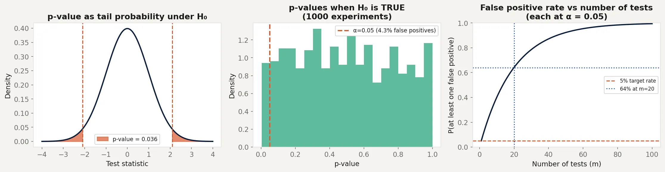
        break

The left panel shows the p-value as the red shaded tail area. The observed statistic of 2.1 gives a p-value of about 0.036. That’s the probability of seeing a statistic this extreme or more, not the probability the null is true.

The middle panel shows what happens when the null is actually true. Run 1,000 experiments on data with no real effect and the p-values are uniformly distributed between 0 and 1. About 5% fall below 0.05, producing false positives. The false positive rate matches α exactly, as it should.

The right panel shows the multiple testing problem. At 20 simultaneous tests, the chance of at least one false positive is 64%. At 100 tests, it’s over 99%. This is why large-scale genetic studies, drug discovery pipelines, and genomics research require corrections like Bonferroni or the false discovery rate.

Business application

A/B testing dashboards. Most A/B testing platforms compute p-values continuously as data arrives and display them in real time. If you stop the test the moment p crosses 0.05, you’re p-hacking. The platform is showing you a number that’s only valid at the predetermined sample size. Early stopping inflates false positives. Sequential testing methods handle this correctly, but they’re less commonly implemented.

Multi-metric experiments. If your A/B test tracks 10 metrics and you declare success when any of them cross p = 0.05, you’re running 10 tests simultaneously. Your actual false positive rate is roughly 40%, not 5%. Either correct for multiple comparisons (Bonferroni: use α = 0.005 per test) or pre-specify which metric is the primary one before running the test.

“We found no significant effect.” A p-value above 0.05 doesn’t mean the null is true. It means you failed to find strong evidence against it. An underpowered study (too few observations) will produce large p-values even when a real effect exists. “Not significant” means “inconclusive,” not “no effect.” The next post on statistical power addresses this directly.

Publication bias and the replication crisis. Scientific journals historically published significant results (p < 0.05) and rejected null results. This created an archive of published findings that overrepresents false positives. When psychology, medicine, and economics researchers tried to replicate published findings in the 2010s, replication rates ranged from 35% to 60%. The p-value wasn’t broken. The incentive structure that selected for p < 0.05 was.