Your sample is lying to you (and how to catch it)

The underlying idea

You want to know the average income of people in your country. You can’t ask everyone, so you ask 1,000 people. If those 1,000 were chosen well, their average income will be close to the true national average. If those 1,000 were chosen badly (say, by surveying people leaving a luxury department store), the result will be wildly wrong. Both samples have 1,000 observations. Both produce a number. Only one is useful.

Sampling is the process of selecting a subset of a population to learn something about the whole. It works because of a mathematical guarantee: if you draw observations at random, the statistics you compute from the sample (the mean, the proportion, the variance) will converge to the true population values as the sample grows. This is the Law of Large Numbers from the probability foundations post.

But “at random” is doing enormous work in that sentence. Most real-world samples are not truly random, and the ways they deviate from randomness are where mistakes happen. Understanding what makes a sample trustworthy, and recognizing when your sample is misleading you, is more important than any statistical test you’ll ever run. A perfect analysis on a biased sample produces a precisely wrong answer.

Historical root

The foundations of sampling theory were laid by Anders Kiaer, a Norwegian statistician who proposed “representative sampling” to the International Statistical Institute in 1895. His idea was controversial: most statisticians at the time believed you needed a complete census to make reliable claims about a population. Kiaer argued that a carefully chosen subset could do the job.

Jerzy Neyman formalized this in 1934 with his paper on stratified random sampling. Neyman showed mathematically that random selection, combined with stratification (dividing the population into groups and sampling from each), could produce estimates with known precision. This paper transformed sampling from an art into a science with provable error bounds.

The most famous sampling failure came in 1936. The Literary Digest magazine mailed questionnaires to 10 million people to predict the U.S. presidential election. They received 2.4 million responses, an enormous sample. They predicted Alf Landon would defeat Franklin Roosevelt in a landslide. Roosevelt won 46 of 48 states. The problem: the magazine drew its mailing list from telephone directories and automobile registrations. In 1936, during the Great Depression, these skewed heavily toward wealthier Americans who favored Landon. Meanwhile, George Gallup correctly predicted the outcome with a sample of just 50,000, chosen to represent the actual voting population.

The lesson has not changed in 90 years: sample size does not fix sample bias.

Key assumptions

For a sample to produce trustworthy estimates of a population, several conditions need to hold. Each one gets violated regularly in practice.

Random selection. Every member of the population must have a known, nonzero chance of being selected. If some members have zero chance (people without internet in an online survey, non-English speakers in an English-only questionnaire), your sample systematically excludes part of the population. This is coverage bias.

Independence of observations. Each selected unit should not influence whether another unit is selected, and the responses should be independent. Violated when you survey households and count every family member (clustered data), or when social influence spreads through a network (one person’s behavior changes another’s).

Sufficient size. Larger samples produce more precise estimates, but the relationship is not linear. Doubling the sample size does not double the precision. Precision improves with the square root of $n$. Going from 100 to 400 observations cuts your margin of error in half. Going from 400 to 1,600 halves it again. This means there are diminishing returns, and beyond a certain point, the cost of more data outweighs the precision gained.

Response and selection effects. Even a perfectly drawn random sample gets distorted if certain people are more likely to respond. Satisfied customers respond to feedback surveys more than dissatisfied ones (or vice versa, depending on the context). People who click on an email survey link are different from those who don’t. This is nonresponse bias, and it can be worse than having a smaller sample.

The math

The core result in sampling theory connects the sample mean to the population mean through the standard error.

If you draw $n$ independent observations from a population with mean $\mu$ and standard deviation $\sigma$, the sample mean $\bar{X}$ has the following properties:

$E[\bar{X}] = \mu$

$\text{SE}(\bar{X}) = \frac{\sigma}{\sqrt{n}}$

The first equation says the sample mean is an unbiased estimator of the population mean. On average, across many possible samples, $\bar{X}$ equals $\mu$. The second equation gives the standard error, which measures how much $\bar{X}$ varies from sample to sample.

The standard error formula reveals the square root relationship between sample size and precision. To cut the standard error in half, you need four times as many observations. This is why pollsters don’t survey millions of people. The precision gained beyond a few thousand is marginal relative to the cost.

For proportions (like conversion rates), the standard error has a slightly different form. If the true proportion is $p$:

$\text{SE}(\hat{p}) = \sqrt{\frac{p(1-p)}{n}}$

This formula reaches its maximum when $p = 0.5$ (maximum uncertainty) and shrinks toward zero as $p$ approaches 0 or 1.

The margin of error reported in polls is typically $1.96 \times \text{SE}$, corresponding to a 95% confidence interval. For a poll of 1,000 people with $p = 0.5$:

$\text{ME} = 1.96 \times \sqrt{\frac{0.5 \times 0.5}{1000}} \approx 0.031$

That’s the familiar “plus or minus 3 percentage points.”

Stratified sampling

When the population has distinct subgroups (strata) that differ on the variable of interest, you can reduce the standard error by sampling from each stratum separately. The stratified estimator is:

$\bar{X}_{\text{strat}} = \sum_{h=1}^{H} W_h \bar{X}_h$

where $W_h$ is the proportion of the population in stratum $h$ and $\bar{X}_h$ is the sample mean within stratum $h$. If the strata are internally homogeneous, the stratified standard error will be smaller than the simple random sampling standard error for the same total $n$.

The code

This script demonstrates three things: how sample size affects precision, how bias distorts results regardless of sample size, and how stratified sampling reduces variance.

import numpy as np
import matplotlib.pyplot as plt

rng = np.random.default_rng(42)

# True population: income is right-skewed (log-normal)
population_size = 100_000
population = rng.lognormal(mean=10.5, sigma=0.8, size=population_size)
true_mean = population.mean()

fig, axes = plt.subplots(1, 3, figsize=(15, 4))

# --- Panel 1: Sample size vs precision ---
sample_sizes = [10, 50, 100, 500, 1000, 5000]
n_repeats = 1000
means_by_size = {}

for n in sample_sizes:
    sample_means = [rng.choice(population, size=n).mean() for _ in range(n_repeats)]
    means_by_size[n] = sample_means

axes[0].boxplot(
    [means_by_size[n] for n in sample_sizes],
    labels=[str(n) for n in sample_sizes]
)
axes[0].axhline(y=true_mean, color="red", linestyle="--", label=f"True mean: {true_mean:,.0f}")
axes[0].set_xlabel("Sample size")
axes[0].set_ylabel("Sample mean")
axes[0].set_title("Precision improves with sample size")
axes[0].legend(fontsize=8)

# --- Panel 2: Bias from non-random sampling ---
# Biased sample: only top 30% of incomes (like surveying luxury shoppers)
biased_pool = population[population > np.percentile(population, 70)]
biased_means = [rng.choice(biased_pool, size=1000).mean() for _ in range(n_repeats)]
random_means = [rng.choice(population, size=1000).mean() for _ in range(n_repeats)]

axes[1].hist(random_means, bins=30, alpha=0.6, label="Random sample", color="steelblue")
axes[1].hist(biased_means, bins=30, alpha=0.6, label="Biased sample", color="coral")
axes[1].axvline(x=true_mean, color="red", linestyle="--", label=f"True mean")
axes[1].set_xlabel("Sample mean")
axes[1].set_title("Bias vs random (both n=1000)")
axes[1].legend(fontsize=8)

# --- Panel 3: Stratified vs simple random ---
# Create 3 income strata
low = population[population < np.percentile(population, 33)]
mid = population[(population >= np.percentile(population, 33)) &
                 (population < np.percentile(population, 66))]
high = population[population >= np.percentile(population, 66)]

n_total = 300
simple_means = []
strat_means = []

for _ in range(n_repeats):
    # Simple random sample
    simple = rng.choice(population, size=n_total)
    simple_means.append(simple.mean())

    # Stratified: 100 from each stratum, weighted by stratum proportion
    s_low = rng.choice(low, size=100)
    s_mid = rng.choice(mid, size=100)
    s_high = rng.choice(high, size=100)
    w_low = len(low) / population_size
    w_mid = len(mid) / population_size
    w_high = len(high) / population_size
    strat_mean = w_low * s_low.mean() + w_mid * s_mid.mean() + w_high * s_high.mean()
    strat_means.append(strat_mean)

axes[2].hist(simple_means, bins=30, alpha=0.6, label="Simple random", color="steelblue")
axes[2].hist(strat_means, bins=30, alpha=0.6, label="Stratified", color="seagreen")
axes[2].axvline(x=true_mean, color="red", linestyle="--")
axes[2].set_xlabel("Sample mean")
axes[2].set_title("Stratified reduces variance (n=300)")
axes[2].legend(fontsize=8)

plt.tight_layout()
plt.savefig("sampling_demo.png", dpi=150)
plt.show()

print(f"True population mean: {true_mean:,.0f}")
print(f"Simple random SE:     {np.std(simple_means):,.0f}")
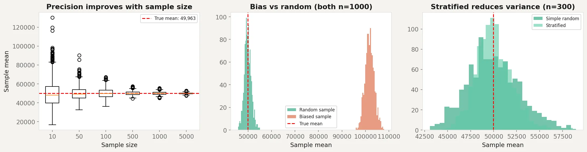
print(f"Stratified SE:        {np.std(strat_means):,.0f}")

The left panel shows how sample means cluster more tightly around the true mean as $n$ increases. At $n = 10$, the estimates are all over the place. At $n = 1000$, they’re tightly concentrated.

The middle panel is the key lesson. Both the random and biased samples have $n = 1000$, but the biased sample (drawn only from the top 30% of incomes) consistently overestimates the true mean. No amount of data fixes this. The distribution of biased sample means doesn’t even overlap with the true mean.

The right panel shows stratified sampling in action. Both approaches use $n = 300$, but the stratified version produces estimates with less variance because it ensures representation from each income group.

Business application

Market research. Online surveys suffer from coverage bias (excludes people without internet access), nonresponse bias (only motivated people respond), and self-selection bias (voluntary opt-in skews toward strong opinions). If you’re surveying product satisfaction, the people who bother to respond are disproportionately either very happy or very unhappy. The silent middle is missing from your data.

A/B testing. Randomization is the entire point of an A/B test. If users aren’t randomly assigned to treatment and control groups, the comparison is invalid. Common violations: letting users self-select into groups, running the test during an unusual period (holiday traffic isn’t representative of normal traffic), or having a technical bug that systematically assigns certain user types to one group.

Clinical trials. The gold standard is the randomized controlled trial precisely because it eliminates selection bias. Patients are randomly assigned to drug or placebo so that the two groups are comparable on every variable, measured and unmeasured. When randomization isn’t possible (observational studies), the door opens to confounders, and the analysis gets much harder.

Machine learning. Train/test splits are a sampling problem. If your training data isn’t representative of the data the model will encounter in production, performance estimates are misleading. Time series data is especially tricky: a random split mixes future data into the training set (data leakage). You need a temporal split: train on the past, test on the future.

When NOT to trust your sample. Be suspicious when: the sample was collected by convenience (surveying whoever is easy to reach), the response rate is low (under 30% is a red flag), the sample was collected during an unusual period, or the population has changed since the data was collected. In all these cases, the sample statistics are precisely computed but wrong. The math is right. The data is not.