Statistical power is why your A/B test found nothing

The underlying idea

Your A/B test ran for two weeks. The new feature showed a 4% lift in conversion. The p-value was 0.18. You declared no effect and moved on.

But what if the effect was real? What if you simply didn’t collect enough data to detect it?

This is the false negative problem, and it’s at least as common as the false positive problem that p-values are designed to control. Statistical power is the probability that your test will detect a real effect when one actually exists. A test with 80% power will miss real effects 20% of the time. A test with 40% power will miss them 60% of the time.

Most A/B tests in practice are severely underpowered. Teams set a significance threshold of 0.05 (controlling false positives) but never calculate power (ignoring false negatives). The result is a graveyard of “no effect” conclusions that were actually inconclusive conclusions from tests that were too small to detect the effect they were looking for.

Understanding power changes how you run experiments. It tells you how much data you need before you start, not after you see the results.

Historical root

Jerzy Neyman and Egon Pearson introduced statistical power in their 1933 paper that also established the hypothesis testing framework. Their key insight was that there are two ways to be wrong in a hypothesis test, and both deserve explicit control.

Type I error (alpha): Rejecting a true null hypothesis. A false positive. The probability of this error is what Fisher’s p-value controls.

Type II error (beta): Failing to reject a false null hypothesis. A false negative. The probability of this error is what power controls. Power = 1 minus beta.

Fisher’s framework focused entirely on controlling Type I error. Neyman and Pearson argued this was incomplete. In their view, you also need to specify the minimum effect size you care about detecting and the acceptable rate of missing it. Without these decisions, you can’t know whether your test is capable of answering your question.

The tension between these frameworks is why most practitioners use a hybrid that specifies alpha (from Fisher) but rarely calculates power (from Neyman-Pearson). The result is a culture that takes false positives seriously and false negatives casually.

Jacob Cohen formalized power analysis for the social sciences in his 1969 book Statistical Power Analysis for the Behavioral Sciences. Cohen surveyed published psychology studies and found most were dramatically underpowered, often with power below 50% for detecting medium-sized effects. His work established the convention of targeting 80% power and introduced effect size measures like Cohen’s d.

Key assumptions

The effect size is specified in advance. Power calculations require you to state the minimum effect you want to detect. A larger effect is easier to detect (requires less data). A smaller effect requires more data. If you don’t know what effect size matters to your business, you can’t calculate the required sample size.

The variability of the outcome is known or estimated. Power depends on the signal-to-noise ratio. The signal is the effect size. The noise is the standard deviation of the outcome variable. Higher variability means you need more data to see the same effect. You can estimate variability from historical data or a pilot study.

The significance level is fixed. Power is calculated for a specific alpha. Lowering alpha (being more conservative about false positives) reduces power for the same sample size. Raising alpha increases power but also increases false positives. These two error rates trade off directly.

The test is two-tailed by default. One-tailed tests have more power for detecting effects in a specific direction, but they completely miss effects in the opposite direction. Most business experiments should use two-tailed tests unless there is a strong prior reason to test only one direction.

The math

For a two-sample t-test comparing means, the required sample size per group to achieve power $1 - \beta$ at significance level $\alpha$ is:

$$n = \frac{2(z_{\alpha/2} + z_{\beta})^2 \sigma^2}{\delta^2}$$

where $z_{\alpha/2}$ is the critical value for the significance level (1.96 for alpha = 0.05, two-tailed), $z_{\beta}$ is the critical value for the desired power (0.84 for 80% power, 1.28 for 90% power), $\sigma$ is the standard deviation of the outcome, and $\delta$ is the minimum detectable effect.

The formula reveals three levers.

To detect a smaller effect ($\delta$ decreases), $n$ must increase quadratically. Halving the minimum detectable effect requires four times the sample size. This is why detecting small improvements is expensive.

To increase power ($z_{\beta}$ increases), $n$ must increase. Going from 80% to 90% power requires roughly 30% more data.

To reduce alpha ($z_{\alpha/2}$ increases), $n$ must increase. Being more conservative about false positives requires more data to maintain the same power.

Cohen’s d standardizes the effect size by the standard deviation:

$$d = \frac{\delta}{\sigma}$$

Cohen’s conventions: small effect d = 0.2, medium effect d = 0.5, large effect d = 0.8. A medium effect requires about 64 observations per group for 80% power at alpha = 0.05. A small effect requires about 394 per group.

The code

import numpy as np
import matplotlib.pyplot as plt
from scipy import stats

rng = np.random.default_rng(42)

# --- Sample size calculation ---
def required_n(alpha, power, delta, sigma):
    z_alpha = stats.norm.ppf(1 - alpha / 2)
    z_beta = stats.norm.ppf(power)
    return int(np.ceil(2 * (z_alpha + z_beta)**2 * sigma**2 / delta**2))

# Business scenario: conversion rate baseline = 10%, detect 2% lift
baseline = 0.10
sigma = np.sqrt(baseline * (1 - baseline))
delta = 0.02

n_80 = required_n(alpha=0.05, power=0.80, delta=delta, sigma=sigma)
n_90 = required_n(alpha=0.05, power=0.90, delta=delta, sigma=sigma)
n_95 = required_n(alpha=0.05, power=0.95, delta=delta, sigma=sigma)

print(f"To detect a {delta:.0%} lift from {baseline:.0%} baseline:")
print(f"  80% power: {n_80:,} per group ({2*n_80:,} total)")
print(f"  90% power: {n_90:,} per group ({2*n_90:,} total)")
print(f"  95% power: {n_95:,} per group ({2*n_95:,} total)")

# --- Power curves ---
sample_sizes = np.arange(10, 500, 5)
for d, label in [(0.2, 'Small (d=0.2)'),
                  (0.5, 'Medium (d=0.5)'),
                  (0.8, 'Large (d=0.8)')]:
    powers = []
    for n in sample_sizes:
        nc = d * np.sqrt(n / 2)
        power = 1 - stats.norm.cdf(1.96 - nc) + stats.norm.cdf(-1.96 - nc)
        powers.append(power)
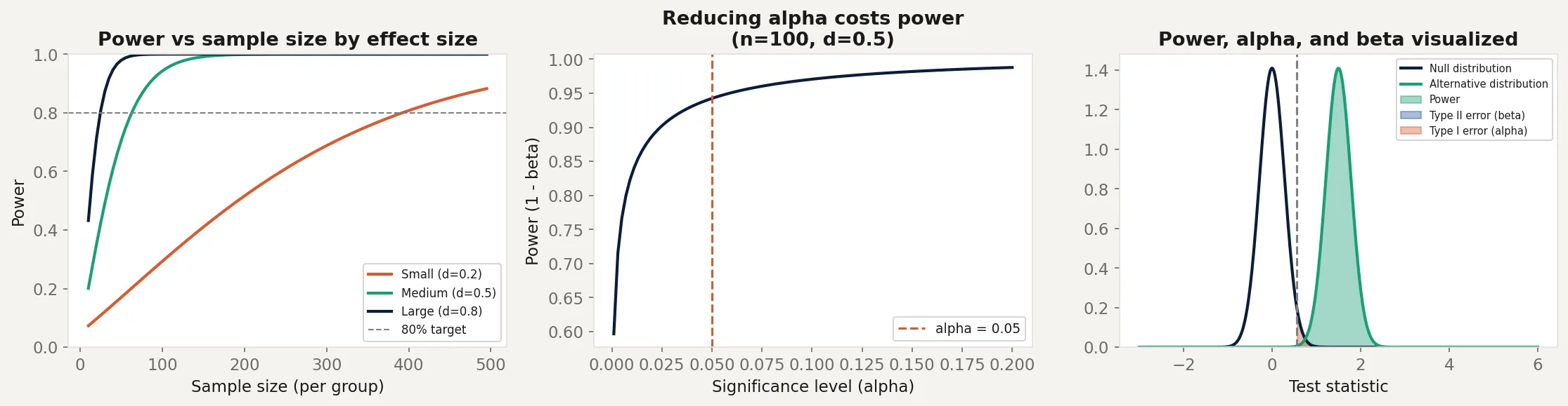
    print(f"{label}: needs n={sample_sizes[next(i for i,p in enumerate(powers) if p >= 0.8)]} for 80% power")

The left panel shows power curves for small, medium, and large effects. A small effect (d = 0.2) needs nearly 400 observations per group to reach 80% power. A large effect (d = 0.8) needs fewer than 30. This is why detecting small improvements in A/B tests is expensive.

The middle panel shows the Type I/Type II error tradeoff. As alpha increases (becoming more lenient about false positives), power increases. You can’t improve both simultaneously with a fixed sample size. More data is the only way to improve both at once.

The right panel shows all three concepts simultaneously. The null and alternative distributions overlap. Power is the green region (correctly rejecting when the alternative is true). Beta is the blue region (missing the effect). Alpha is the red region (falsely rejecting the null).

Business application

Pre-experiment planning is the only honest approach. Before running an A/B test, calculate the required sample size based on your baseline metric, the minimum lift you care about, and your target power. If you can’t reach that sample size in a reasonable time, the test won’t answer your question. Running it anyway and declaring “no effect” is not valid inference. It’s an inconclusive experiment presented as a conclusion.

Choosing the minimum detectable effect (MDE). The MDE is a business decision, not a statistical one. A 0.1% conversion lift on $100M revenue is $100K annually. Worth detecting. A 0.1% lift on $50K revenue is $50. Probably not worth a long experiment. Set the MDE based on what difference would actually change your decision, then let statistics tell you how much data that requires.

Underpowered studies in medical research. Cohen’s 1962 survey of psychology journals found average power of roughly 46% for medium effects. More recent analyses of clinical trials have found similar patterns, with many trials too small to reliably detect clinically meaningful differences. An underpowered trial that finds p greater than 0.05 doesn’t prove a treatment doesn’t work. It proves the study couldn’t tell either way.

Sequential testing as an alternative. Fixed-sample power analysis requires you to commit to a sample size before seeing any data and not peek until you’re done. This is operationally difficult. Sequential testing methods (like SPRT or always-valid confidence intervals) allow continuous monitoring with controlled error rates, at the cost of slightly larger required samples. These are increasingly available in A/B testing platforms and are worth understanding for high-velocity experimentation.